Fourier transforms can see the future

Motivation

Consider the ODE for a driven harmonic oscillator with no dissipation:

$$\boxed{\ddot x + \omega^2 x=f(t),\quad x(0)=x_0,\quad \dot x(0)=v_0,}\tag{1.1}$$

where we pick $f$ to be completely generic.

One approach we may attempt in order to solve this equation is to use Fourier transforms. By writing $x(t)$ as

$$x(t)=\int_{-\infty}^\infty \frac{dk}{2\pi}\; e^{ikt} \widetilde x(k)$$

we see that time derivatives will just bring out factors of $ik$ from the exponent. We write the analogous expression for $f$ as an integral of $\widetilde f(k)$, and obtain

$$\int_{-\infty}^\infty \frac{dk}{2\pi} e^{ikt} (-k^2+\omega^2) \widetilde x(k) = \int_{-\infty}^\infty \frac{dk}{2\pi} e^{ikt} \widetilde f(k).$$

From the orthogonality of the Fourier basis, this will hold only if

$$(-k^2+\omega^2)\widetilde x(k)=\widetilde f(k) \implies \widetilde x(k)=\frac{\widetilde f(k)}{\omega^2-k^2}.$$

Unfortunately for us, this expression has singularities at $k = \pm\omega$. The inverse transform, given by

$$x(t)=\int_{-\infty}^\infty \frac{dk}{2\pi}\; e^{ikt} \widetilde x(k)=\int_{-\infty}^\infty \frac{dk}{2\pi} e^{ikt} \frac{\tilde f(k)}{\omega^2-k^2}$$

is therefore ill-defined. This is the first issue with this approach.

The second issue comes from the intermediate calculation of the Fourier transform of $f$, namely

$$\tilde f(k) = \int_{-\infty}^\infty dt \; e^{ikt} f(t),$$

for which we need information about $f(t)$ for all times, including future times relative to our evaluation point. This seems to violate our physical intuition that the response at time $t$ should only depend on the forcing for times $t' \leq t$, which means our approach does not seem to preserve causality.

In what follows, I will present three ways to deal with these issues and solve this system. We will then see how different approaches tackle the issues of causality and divergence, and how all converge to the same answer.

Notice that the general solution to the inhomogeneous system (1.1) is the general solution of the homogenous equation, plus a specific solution $x_p$ to the inhomogeneous one:

$$\boxed{x(t) = A \sin \omega t + B\cos \omega t + x_p(t).}\tag{1.2}$$

We will mostly focus on finding $x_p(t)$.

The basic approach: variation of parameters

As a linear differential equation with constant coefficients, we can tackle this equation with standard methods, and particularly with the method of variation of parameters.

Recall the method for a second-order equation: given two linearly independent solutions $u_1(t)$ and $u_2(t)$, we seek a solution to the inhomogeneous equation of the form

$$x_p(t) = A(t) u_1(t)+B(t) u_2(t)$$

where $A(t)$ and $B(t)$ are currently undetermined. Since we have two unknowns, we can add a constraint between them to close the system; a convenient one is

$$\dot A(t) u_1(t) + \dot B(t) u_2(t) = 0 \quad\forall t$$

since it also simplifies a lot the algebraic manipulations. As the Wikipedia page derives, one can then find explicitly the functions $A$ and $B$ as any indeterminate integrals

$$A(t) =- \int^t \frac{1}{W(t')} u_2(t') f(t') dt',\quad B(t)=+\int^t\frac{1}{W(t')} u_1(t') f(t') dt'$$

where

$$W(t) = \det \begin{bmatrix} u_1(t) & u_2(t) \\ \dot u_1(t) & \dot u_2(t) \\ \end{bmatrix}$$

is the so-called Wronskian determinant. The lower limit of the integrals can be chosen at will - their choice is basically that of two arbitrary constants. These will contribute to the solution a factor of $\mathrm{const}_1 u_1(t) + \mathrm{const}_2 u_2(t)$ which can be absorbed into the constants in (1.2). For now, let us set it to be a number $t_0$, to be determined.

For the harmonic oscillator, one has

$$u_1(t) = \cos \omega t,\quad u_2(t)=\sin \omega t$$

from which follows that $W = \omega$ and then

$$A(t) = -\int_{t_0}^t \frac{\sin \omega t'}{\omega} f(t') dt',\quad B(t)=\int_{t_0}^t \frac{\cos \omega t'}{\omega} f(t') dt'.$$

Now, we construct the solution $x_p(t) = A(t) u_1(t)+B(t) u_2(t)$ as

$$\begin{align*} x_p(t) &= - \cos \omega t\int_{t_0}^t \frac{\sin \omega t'}{\omega} f(t') dt' + \sin \omega t\int_{t_0}^t \frac{\cos \omega t'}{\omega} f(t') dt'\\ &=\frac 1\omega \int_{t_0}^t dt'\;f(t') [\sin \omega t \cos \omega t'-\sin \omega t'\cos \omega t] \end{align*}$$

or, simplifying,

$$\boxed{x_p(t)= \frac 1 \omega \int_{t_0}^t \sin \omega(t-t') f(t') dt'.}\tag{2.1}$$

Substituting this in (1.2) yields

$$x(t) = C \sin \omega t + D\cos \omega t + \frac 1 \omega \int_{t_0}^t \sin \omega(t-t') f(t') dt'$$

with three arbitrary constants: $C, D$ and $t_0$.

We now plug in the initial conditions $x(0) = x_0$, $\dot x(0) = v_0$. Using the fundamental theorem of calculus in the form

$$\frac{d}{dt}\int_{a(t)}^{b(t)} g(t,s) ds=g(t,b(t))-g(t,a(t))+\int_{a(t)}^{b(t)} \frac{\partial g}{\partial t}(t,s) ds$$

we obtain

$$\begin{align*} x_0 &=D -\frac 1 \omega \int_{t_0}^0 \sin \omega t' \;f(t')dt'\\ v_0 &= \omega C + \left[0+ \frac 1 \omega\int_{t_0}^0 \omega \cos \omega t'\; f(t') dt'\right] \end{align*}$$

Notice that, by setting $t_0=0$, the integrals vanish and we find a solution $D = x_0$, $C = v_0/\omega$. Hence, we can write our final solution as

$$\boxed{x(t) = x_0 \cos \omega t + \frac{v_0}{\omega}\sin \omega t + \frac 1\omega \int_0^t \sin\omega(t-t')\,f(t') dt'.}$$

Approach 1: Green’s function

Given an inhomogeneous differential equation, schematically written

$$Lu=f$$

(where $L=L(t)$ is a differential operator and $u$ is the solution we seek), we define the Green’s function $G = G(t,t')$ for the operator $L$ as the distribution satisfying the same equation, but with the right-hand side formally replacing $f$ with a delta function:

$$LG(t,t') = \delta(t,t')$$

If the system displays time-translation invariance, then $G$ is just a function of the time difference $t-t'$ and so

$$L G(t-t') = \delta(t-t').$$

I now claim that the convolution

$$u(t) = \int_{-\infty}^\infty G(t,t') f(t')dt'\tag{3.1}$$

is the desired solution to $Lu=f$:

$$Lu(t)=\int_{-\infty}^\infty [LG(t,t')] f(t')dt'= \int_{-\infty}^\infty \delta(t-t') f(t')dt'=f(t).$$

It follows that our problem, (1.1), can be solved by direct integration if we can find $G$ satisfying

$$\ddot G(t)+\omega^2 G(t)=\delta(t).\tag{3.2}$$

Now, Green’s functions are usually not unique; if $u_0$ is a solution to the homogeneous equation, then $G + u_0$ is a valid Green’s function. We may, therefore, seek a causal Green’s function that satisfies $G(t-t') \neq 0$ only if $t > t'$, and zero otherwise, since in this case (3.1) becomes

$$u(t) = \int_{-\infty}^t G(t-t') f(t') dt'$$

only depending on information available before time $t$.

Note: in physics, one often calls such $G$ the retarded Green’s function. One could also do the opposite, and seek $G$ that is zero for all times later than the present (and advanced Green’s function).

We thus find our first “boundary condition” on $G$: $G(t-t') = 0$ for all $t' > t$, or equivalently

$$G(t) = 0\quad\text{ for all } t<0.\tag{3.3}$$

Secondly, we can directly integrate (3.2) between $[-\epsilon, \epsilon]$, for small $\epsilon > 0$, yielding

$$\dot G(\epsilon)-\dot G(-\epsilon) + \omega^2 \int_{-\epsilon}^\epsilon G(t)dt = 1.$$

If we assume $G$ to be continuous, then in the limit $\epsilon \to 0^+$ the integral vanishes. (3.3) further implies $\dot G(-\epsilon) \to 0$, and hence we find the second boundary condition:

$$\dot G(0^+) = 1.\tag{3.4}$$

Notice how the delta function introduces a discontinuity in the first derivative at $t=0$.

We now rephrase problem (3.2) as

$$\boxed{\ddot G(t)+\omega^2 G(t)=\delta(t) \quad \text{ for } G \text{ continuous, with } G(t) = 0,\; t< 0 \text{ and } \dot G(0^+)=1.}$$

The strategy to find $G$ is to realize that, for $t> 0$, the delta function vanishes and we have to solve the equation for a free harmonic oscillator:

$$\ddot G(t)+\omega^2 G(t)= 0,\; t>0 \quad\implies \quad G(t)=A\cos \omega t+B \sin \omega t.$$

Now, we impose the conditions. Continuity at $t=0$ requires

$$G(0^+) = 0 \implies A = 0.$$

The condition on the first derivative yields

$$\dot G(0^+) = \omega B = 1 \implies B=\frac{1}{\omega}.$$

Hence, we find

$$\boxed{G(t)=\frac{\sin \omega t}{\omega} \boldsymbol 1_{t \geq 0}}\tag{3.5}$$

and the particular solution is thus

$$x_p(t) = \int_{-\infty}^\infty G(t-t')f(t')dt'=\frac{1}{\omega}\int_{-\infty}^t \sin \omega(t-t') f(t')dt',$$

same as (2.1).

Green’s function from variation of parameters

From the variation of parameters formulas, we can actually obtain the Green’s function as well. Recall that we had two independent solutions of the homogenous equation, $u_1(t)$ and $u_2(t)$, and we tried to write a specific solution to the inhomogeneous equation as

$$x_p(t)=A(t) u_1(t)+B(t)u_2(t)$$

with

$$A(t) =- \int^t \frac{1}{W(t')} u_2(t') f(t') dt',\quad B(t)=+\int^t\frac{1}{W(t')} u_1(t') f(t') dt'.$$

We can write this in full as

$$x_p(t)=\int^t \left[\frac{u_1(t')u_2(t)-u_1(t) u_2(t')}{W(t')} \right]f(t') dt'.$$

Comparing this to (3.1), we can read off the Green’s function as

$$\boxed{G(t,t')=\frac{u_1(t')u_2(t)-u_1(t) u_2(t')}{W(t')}}$$

In our case, with $W = \omega$ and $u_1(t) = \cos \omega t$, $u_2(t) = \sin \omega t$, this yields

$$G(t,t')=\frac{1}{\omega}(\sin \omega t \cos \omega t'-\sin \omega t'\cos \omega t)=\frac{\sin \omega(t-t')}{\omega}$$

which is the correct expression. Note that this expression is defined for all $t, t'$, but the retarded Green’s function requires $G(t,t') = 0$ for $t < t'$. In the variation of parameters derivation, causality is enforced not by $G$ itself but by the upper limit of integration $\int^t$, which restricts $t' \leq t$. To make the connection with (3.5) explicit, one should write

$$G(t,t') = \frac{\sin \omega(t-t')}{\omega}\,\boldsymbol 1_{t \geq t'}.$$

Approach 2: Laplace transform

The Laplace transform is a general tool for analyzing dynamical systems. Its usefulness for us stems mostly from how it is automatically causal.

For a function $f$, its Laplace transform is

$$\widehat f(s)\equiv\mathcal L\{f\}(s) = \int_{0^-}^\infty f(t) e^{-st} dt\tag{4.1}$$

for $s \in \mathbb C$. Integration by parts gives the usual rule for the derivative transform:

$$\mathcal L \{\dot f \}(s) = s \widehat f(s)-f(0^-)$$

and applying this rule once more gives

$$\mathcal L \{\ddot f \}(s) = s^2 \widehat f(s)- s\dot f(0^-) -f(0^-)$$

The fact that the lower limit of integration is $0^-$ means that the support of the standard delta function $\delta(t)$ is contained in the domain of integration, and so one finds

$$\mathcal L\{ \delta \}(s)=\int_{0^-}^\infty \delta(t) e^{-st} dt = 1.$$

We are thus able to take the transform of (3.2), i.e. $\ddot G(t)+\omega^2 G(t)=\delta(t)$, as

$$s^2\widehat G(s)-s \dot G(0^-) - G(0^-) + \omega^2 \widehat G(s) = 1.$$

Now, we have seen that $G(0^-) = \dot G(0^-) = 0$, so these terms vanish from the left-hand side. We find

$$\widehat G(s)=\frac{1}{s^2+\omega^2}.\tag{4.2}$$

For the inverse, we cheat and use a lookup table for common Laplace transforms. Wikipedia says that

$$\frac{\omega}{s^2+\omega^2} \text{ is the transform of } \sin \omega t \;\boldsymbol 1_{t\geq 0},$$

so we immediately find

$$G(t)=\frac{\sin \omega t}{\omega} \boldsymbol 1_{t \geq 0}$$

exactly like in (3.5).

Approach 3: back to the Fourier transform

This is by far the hardest and most error-prone approach for this equation, but its discussion is nonetheless interesting.

As we mentioned in the introduction, by taking the Fourier transform of the original equation, we have obtained the Fourier-space equation

$$(-k^2+\omega^2)\widetilde x(k)=\widetilde f(k)$$

which is ill-defined at $k=\pm \omega$. We tackle this now.

For consistency, since we discussed Green’s functions in the two previous sections, we will do the same here; then, instead of $x$ and $f$ we consider $G$ and $\delta$, the latter whose Fourier transform is

$$\widetilde \delta(k) = \int_{-\infty}^\infty dt \; e^{-ikt} \delta(t) = 1.$$

Therefore, in Fourier space, the Green’s function is

$$\widetilde G(k)= \frac{1}{\omega^2 - k^2}$$

(which of course still has the same singularities) and the inverse transform is thus

$$G(t) = \int_{-\infty}^\infty \frac{dk}{2\pi} \;e^{ikt} \widetilde G(k) = \int_{-\infty}^\infty \frac{dk}{2\pi} \frac{e^{ikt}}{\omega^2-k^2}.\tag{5.1}$$

Anyone who has studied complex analysis will recognize this integral as a potential candidate for contour integration. We would like to promote $k$ into a complex number $z$ and consider a closed contour, parameterized by a radius $R > 0$, such that the original integral becomes the limiting case of the integral over the real line segment $[-R, R]$ of the contour, and with the integral over the remaining contour vanishes as $R \to \infty$. Then, the residue theorem allows us to obtain a finite integral.

The issue is then, of course, that the contour currently goes straight over the poles $\pm \omega$. We need some sort of adjustment, either at the circuit level (making it turn around the poles) or at the pole level (shifting their position).

Let us consider a slightly different problem: consider our differential equation but with an added dissipation term:

$$\ddot x +\epsilon \dot x + \omega^2 x=f(t).$$

We expect (hope) that we can solve the equation for $\epsilon \neq 0$ and then take the limit $\epsilon \to 0^+$.

Now, by replacing $f(t)$ with $\delta(t)$ and taking the transform, we arrive at the following expression for the Green’s function:

$$\widetilde G(k)=\frac{1}{\omega^2-k^2+i\epsilon k}.$$

The Green’s function in time domain is then given by the transform

$$G(t)=\int_{-\infty}^\infty \frac{dk}{2\pi} \frac{e^{ikt}}{\omega^2-k^2+i\epsilon k}.$$

We want to tackle this integral via contour integration, formally replacing the real $k$ with a complex number $z$ . The poles are now the complex solutions of $\omega^2-z^2+i\epsilon z=0$, or

$$z_\pm = \pm\omega+\frac{i\epsilon}{2} + O(\epsilon^2).$$

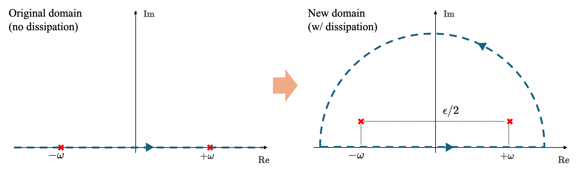
We see that both roots now live in the upper half-plane, at a distance $\epsilon/2$ of the real axis.

Where should we close the contour? If we split $z$ into its real and imaginary parts as $z = \alpha+i\beta$, the exponential is

$$e^{izt}=e^{i\alpha t} e^{-\beta t}.$$

There are two cases to consider:

• If $t \geq 0$, then the exponent $e^{-\beta t}$ will not diverge if $\beta$ is restricted to be positive, or equivalently, if $z$ lives in the upper half-plane. In other words, we should close the circuit on the upper half-plane for $t \geq 0$, and since the poles are contained in this region, the integral will be non-zero (see figure below)

• If $t < 0$, then we need $\beta < 0$ too, and the integral should be done in the lower half-plane. In this case, no poles are contained within the integration contour, and the integral is zero.

We have thus found that

$$G(t) = 0\quad \text{if } t < 0,$$

i.e. causality is immediately satisfied as long as there is even a slight dissipation factor $\epsilon$.

We can now proceed to calculate the integral via the residue theorem. Let $C_R$ denote the half-circle in the picture above, with radius $R$, and abbreviate

$$h_\epsilon(z)= \frac{e^{izt}}{\omega^2-z^2+i\epsilon z}=-\frac{e^{izt}}{(z-z_+)(z-z_-)}.$$

Then, we have

$$\begin{align*} t\geq 0: \quad G(t)&=\int_{-\infty}^\infty \frac{dz}{2\pi} \frac{e^{izt}}{\omega^2-z^2+i\epsilon z}\\ &=\lim_{\epsilon \to 0^+}\lim_{R\to\infty} \frac{1}{2\pi}\int_{C_R} h_\epsilon(z) dz\\ &= \lim_{\epsilon \to 0^+} \frac{1}{2\pi} \cdot2\pi i \Big[\mathrm{Res}\; h_\epsilon \Big\vert_{z=z_+} + \mathrm{Res}\; h _\epsilon\Big\vert_{z=z_-} \Big], \end{align*}$$

where, for a simple pole like $z_+$,

$$\mathrm{Res}\; h_\epsilon \Big\vert_{z=z_+}=\lim _{z\to z_+}(z-z_+)h_\epsilon(z).$$

The calculation is straightforward:

$$\mathrm{Res}\; h_\epsilon \Big\vert_{z=z_+}=\lim _{z\to z_+} \frac{-e^{itz}}{z-z_-}=-\frac{e^{-i\epsilon/2} e^{i\omega t}}{2\omega}$$

and

$$\mathrm{Res}\; h_\epsilon \Big\vert_{z=z_-}=\lim _{z\to z_-} \frac{-e^{itz}}{z-z_+}=+\frac{e^{-i\epsilon/2} e^{-i\omega t}}{2\omega}.$$

Putting all this together and taking the limit $\epsilon \to 0^+$ yields

$$t\geq 0: \quad G(t) = - \lim_{\epsilon \to 0^+}\frac{i e^{-i \epsilon/2}}{2\omega} (e^{i\omega t}-e^{-i\omega t})=\frac{\sin \omega t}{\omega},$$

or equivalently, $G(t) = (1/\omega) \sin \omega t \,\boldsymbol 1_{t \geq 0}$ as obtained previously.