The problem
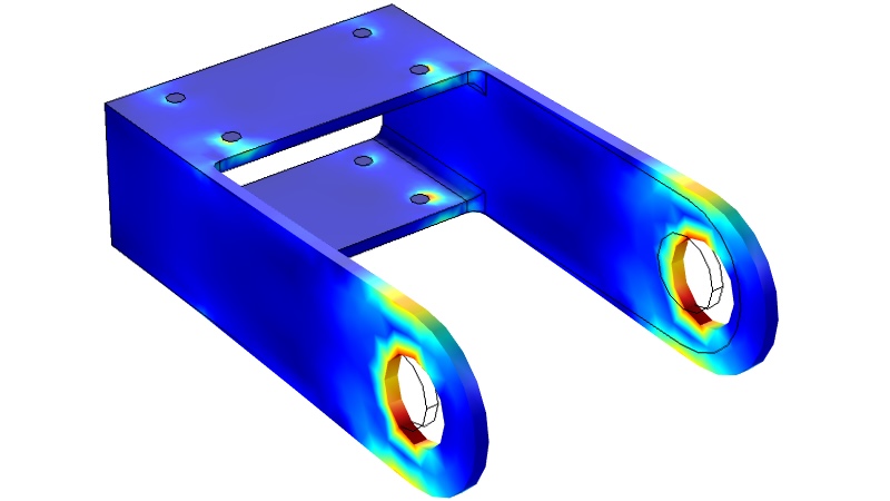
When subject to an increase in temperature, a solid object will usually expand, and this expansion will act to increase internal stresses. In this way, variations in temperature affect solids’ mechanical properties.
On the other hand, inside a solid body, heat transfer occurs mostly by diffusion from hot to colder zones. This depends not only on the temperature gradients, but also on the body’s geometry. Hence, the thermal conductivity and static elasticity problem are coupled.
In many multiphysics applications, one decouples this system by solving it sequentially:
- First solving the heat equation, thus obtaining a temperature profile ;
- Then plugs in this temperature to a thermal stress term in the linear elastic equations, and solves them for the displacement field , which can then be used to derive strains, stresses etc.
In this article we justify why one may decouple the problem in this form in the specific case of solids. We will mostly follow the classical text [1] of Landau & Lifschitz. Throughout the text we employ the Einstein convention of summing over repeated indices.
Recap: the stress tensor and free energy
We follow [1], in which the primary quantity that we consider is the Helmholtz free energy of a solid under deformation. We present the rationale for choosing Helmholtz free energy below.
Tl:DR: The Helmholtz free energy appears as a shortcut to obtain the stress tensor. If we can write , i.e. the free energy as a function of strain, then the stress tensor can be calculated immediately by differentiation, i.e. is the generating function of stress and strain.
By considering virtual displacements, it is not hard to show that the work done by the system if it contains stresses and strains is , per unit volume
where is the stress tensor and is the infinitesimal strain tensor. This equation generalizes the term for work when we only consider pressure.
Then, for a reversible process, we have the first law of thermodynamics in the form
if there are no other work terms; here, is the internal energy and the entropy, both per unit volume. The Helmholtz free energy per unit volume can then be introduced, and its differential is
from which one immediately obtains
Thus, if one can express as a function of the (kinematic) variable . then we can obtain the (dynamic) stress tensor by pure differentiation.
Linear elasticity at constant reference temperature
One obtains (isotropic) linear elasticity by suitably expanding the free energy in terms of the strain tensor .
First, we fix a reference temperature such that we can set the body to be undeformed at this temperature. All quantities in this section are assumed to be evaluated at ; this will be dropped in the following sections.
Since , there must not be any terms linear in in the expansion of , for if there were, then would not be zero.
Now we consider higher order terms. Since is a scalar, all the terms in the expansion must be scalars, meaning they must be (1) number-valued functions and (2) invariant under rotations. For a symmetric matrix there are two rotation-independent quadratic invariants: and ; since is symmetric, we assume with no loss of generality that
or, in index notation
and are, of course, the Lamé coefficients, in units of pressure. We see that they naturally appear as expansion coefficients for the Helmholtz free energy. Notice that, by straightforward differentiation, one finds
which is the usual constitutive law for isotropic linear elasticity.
Adding temperature
If we set a temperature , we expect there to be deformations even in the absence of external forces. Hence, a linear term in must appear in the free energy expansion. Requiring isotropy, the only possible scalar is its trace , thus must contain a term of the form
Assuming temperature variations around to be small, we can expand the coefficient to first order,
Above, we chose to write the coefficient of , with no loss of generality, as the bulk modulus times a factor which is yet to be determined. This is a convenient choice since has units of pressure, and the free energy per unit volume has units of energy/volume = pressure as well. Since is unitless, we conclude has units of inverse temperature.
We have also chosen the constants to not depend on ; if they did, since they cannot have dependence but only , their contributions would only come at higher orders and thus can be ignored.
Again, by differentiation, we find
To understand the effect of this new thermal stress term, assume a body not subject to external forces, just undergoing a change in temperature. The body will deform, so , but there are no stresses, hence . Setting above, we can solve for by contracting indices:
using that . Recalling that is the relative volume increase due to displacement, we see that is the (volumetric) thermal expansion coefficient of the body, which we expect to be positive in order for and to have the same sign.
How the linear elastic equation changes
Recall the equations for a linear elastic body are
where is a bulk force (per unit volume). This equation must be supplemented by initial and boundary conditions.
By writing out as in Eq. (3), we can expand this equation as
where are Young’s modulus and Poisson’s ratio, respectively, and is the displacement field. The denotes how temperature gradients affect the linear elastic equation.
We must complement this equation with one for the temperature field, i.e. the heat equation.
Deriving the heat equation
In solids, in contrast to fluids, internal convection is not an efficient mechanism for heat transfer. Ignoring radiation, whose effects are usually small, we see that heat diffusion is the only mechanism to consider in the interior of a solid body (this is not the case for the body’s interface with an external medium, like a fluid — convection plays an important role here, but this enters as a boundary condition).
Hence, heat flux can be written from Fourier’s law as
where the heat flux vector has units of power per unit area, i.e. energy per unit area per unit second, and is the body’s thermal conductivity. Assume a volume is at a lower temperature than its surroundings; then, it will absorb heat. From the divergence theorem, the total heat absorbed per unit time is, in the absence of a volumetric source/sink term,
The right-hand side is positive since points outward, and the divergence of such a field is positive.
If we wanted to consider a heat source, we would need to add a on the RHS, where has units of power per unit volume. This term would be added to the RHS of equations (5), (7) and (9).
We can write the left-hand side as a function of entropy per unit volume as
from which we derive
Now, we want to get rid of entropy to find an equation for . This can be done as follows. First, remember that, from Eq. (1), we had
it follows that
so we can compute the entropy directly from the free energy. Using Eq. (2), which we repeat here ignoring higher-order terms,
we immediately find
where . Entropy increases as the body expands, which is intuitive. Substituting this into Eq. (5) yields
where we explicitly wrote in terms of the displacement field .
To further simplify this equation, we need a few ingredients. First, Mayer’s relation in the form
where is the thermal expansion coefficient and is called the isothermal compressibility. We can rewrite this as
which is the term multiplying in the equation; hence
We note that
Now, recall the following fact from thermodynamics. At constant volume, one can relate heat and temperature variation as
or, per unit volume, and writing ,
At constant volume, i.e. when , is just (from Eq. (6)) so we can finally rewrite Eq. (8) as
and thus we obtain the full heat equation from (7):
Putting both equations together
Below, we repeat equations (4) and (9), with a little massaging:
From the presence of and in both equations, we see that the two systems are coupled and, in principle, would need to be solved jointly.
What about decoupling?
Case 1: static solutions
Let us assume steady state, where both and have no time dependence. Then, all time derivatives vanish and we are left with
Conveniently, we have no more dependence in the heat equation, which can then be solved directly and its result can be plugged into the linear elastic equation as an effective additional force. This justifies the approach we usually see, i.e. first solving the heat equation and then using its result as an additional “force” in the linear elastic equation.
Case 2: comparing scales
The coupling appears inside the heat equation via the term
which, as we will argue, is usually small: and are very close for solids, and so this term is often completely neglected.
First, from the fact that , we conclude that the two terms in the LHS of the heat equation are
Our comparison then becomes on the scales of
Let us compare these terms:
For some common materials at 300 K, we see that indeed the term multiplying is around < 5% of the first one:
| Material | (in ) | (in ) | (in ) | (in SI units) | (in SI units) | ratio |
|---|---|---|---|---|---|---|
| Aluminum | 69.0 | 0.01385 | 2.422 | 2,422,000 | 103,126 | 4% |
| Copper | 49.9 | 0.0073 | 3.45 | 3,450,000 | 102,329 | 3% |
Because of this, we can mostly neglect this term and stay with the decoupled heat equation
whose result can then be plugged back into the linear elastic equation.
Conclusion
We have seen that, although theoretically coupled, when considering small displacements and small variations in temperature, we can rewrite thermoelastic coupling into a sequential coupling where the heat equation is solved first, and its result is fed into the linear elastic equation.
References
[1]L. Landau, L. Pitaevskii, E. Lifshitz, and A. Kosevich. Theory of Elasticity. Course of Theoretical Physics Volume 7. Butterworth-Heinemann, 3 edition, (1986)